The roofline model [1] identifies and visualizes performance bottlenecks. The plot below shows an example of a roofline plot. It depicts the measured performance of three hypothetical applications appA, appB, and appC against their operational intensity. The roofline model then adds two performance bounds associated with both the computational throughput and the memory bandwidth. The roofline model clearly identifies bottlenecks due to the computational throughput (appA) and the memory bandwidth (appC). However, the original model is inherently blind to bottlenecks due to non-throughput resources such as cache capacity, latency of memory accesses or the functional units, and out-of-order (OoO) execution buffers. For appB, for example, the bottleneck is undetermined.
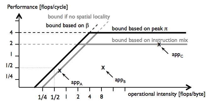
Figure 1: Roofline plot [1].
ERM leverages the detailed per-cycle analysis of the scheduled DAG to associate execution cycles (runtime components like T_issue, T_lat) with hardware resources, and turn them into hardware-related performance bounds that can be included as additional tighter bounds on the roofline plot to provide deeper insights into why peak performance is not reached.
The issue bottleneck is the performance penalty that results from not fully utilizing the throughput ignoring latency-, stall- and overlap-related effects. We model the issue performance bound associated with a node type as the maximum achievable performance if execution consisted only of issue cycles (T_issue), P_issue = W/T_issue.
Figure 2 shows an example of an scheduled DAG and the corresponding roofline plot for L1 cache. The peak performance of the platform is 2 flops/cycle. For the arithmetic nodes (M and A), T_issue is 4 cycles (cycles 12, 14, 21, and 24) which yields a performance bound of P_issue_comp = 1 flop/cycle. This new performance bound is represented as a horizontal line at P = 1 flop/cycle, lowering the original computation bound based on peak computational throughput�. A similar analysis yields the issue performance bound associated with L1 accesses, which is a line parallel to the original L1 memory bandwith bound.
These bounds can be interpreted as follows: Even if there was perfect overlap and no latency or stall-related effects, the maximum achievable performance is 1 flop/cycle due to an underutilization of �the throughput resource. Equivalently, it means that the issuing of floating-point operations is a bottleneck because it reduces the maximum achievable performance.
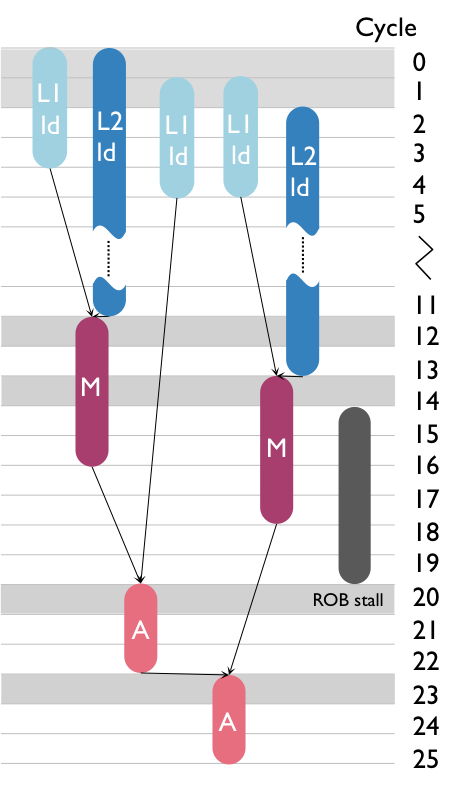
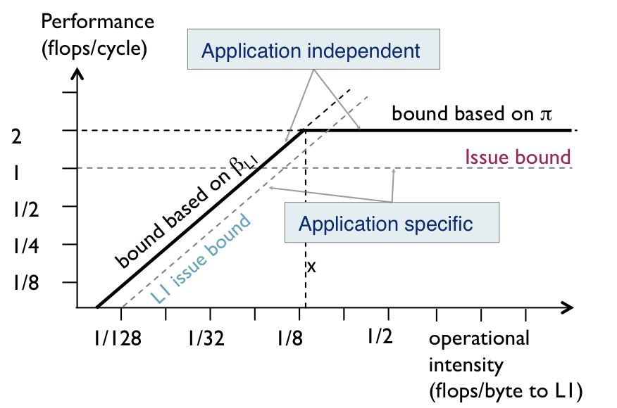
Figure 2: Adding issue performance bounds into the roofline plot.
The latency bottleneck quantifies the performance loss due to latency-only cycles, i.e., cycles in which execution is stalled due to dependences with long-latency operations. In the scheduled DAG in Figure 3, for example, cycles 13, 15–18, 22–23 and 25–26 are idle cycles due to the latency of the arithmetic computations.
For the DAG in Figure 3, T_issue of arithmetic nodes is 4 cycles, T_lat is 9 cycles, and thus P_lat is 0.301 flops/cycle. That is, even ignoring stall effects, memory time, and overlap (these effects are explained later), the maximum achievable performance is 0.301 (out of the 2 flops/cycle provided by the platform) due to the issue and latency effects of the floating-point computations. We represent this bound as a horizontal roof at P = 0.301 flops/cycle.
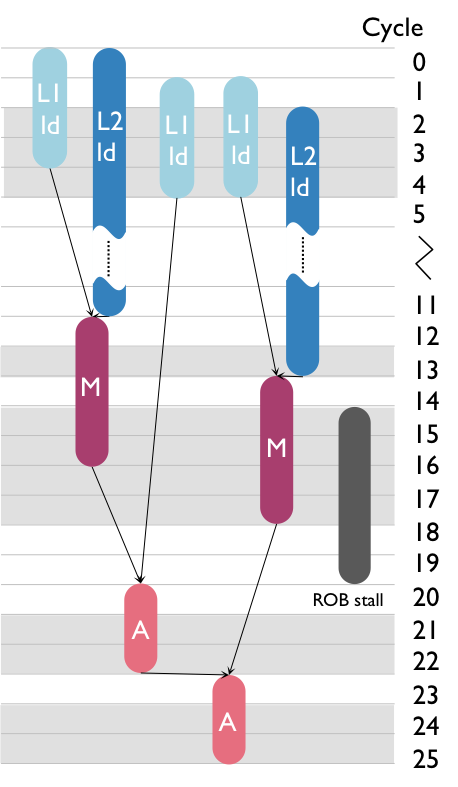
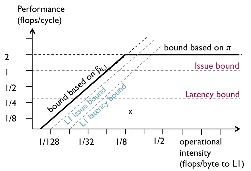
Figure 3: Adding latency performance bounds into the roofline plot.
The stall bottleneck quantifies the fraction of execution time in which buffers are full. In the ERM's DAG-based performance model, these cycles are quantified by the stall times.
Stall nodes, as opposed to computation and memory nodes, do not correspond one-to-one to any of the existing roofs in the roofline plot. To include them into the roofline plot, we consider a runtime component that combines both cycles of a given node type and cycles of a specific stall. As with the latency bound, we define the stall bound taking the issue bound as a reference;
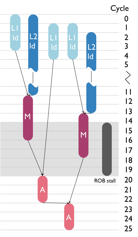
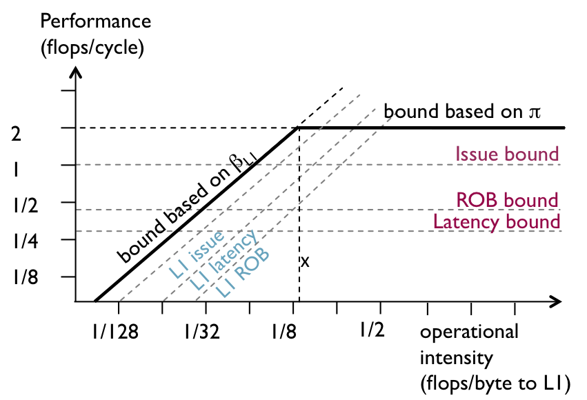 Figure 4: Adding stall performance bounds into the roofline plot.
The overlap bottleneck quantifies the loss of performance due to imperfect overlap between compute and memory nodes. In contrast to the previous bottlenecks, it is defined for pairs of node types including pairs of memory nodes If there is not perfect overlap, the bound yields a curved roof as shown in Figure 4 for our running example. This roof now is tight, i.e., hits the performance point, which shows that the lack of overlap between computation and accesses to L2 is the main reason why peak performance is not reached (as one can confirm by inspecting Fig. 4.2(a)).

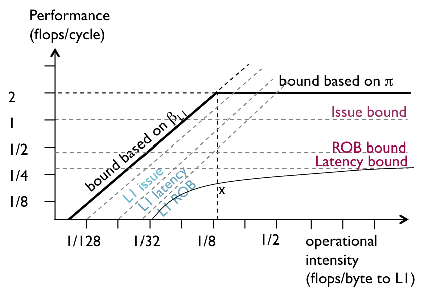
Figure 4: Adding overlap performance bound into the roofline plot.
We redefine operational intensity as flops per byte transferred to all levels of the memory hierarchy. With this new definition of operational intensity we can now create a single roofline plot for all levels of the memory hierarchy, using I as the variable in the x-axis. Note that there is one fundamental difference to the original roofline plot. Because of the factor Q/Qx, the memory bounds in the generalized roofline plor now also depend on program and input.
The result of the previous analysis is a generalization of the roofline plot that integrates all derived bottlenecks as bounds into a single viewgraph. This representation has some limitations, but first we emphasize the following properties of the generalized roofline plot:
-
Progressively tighter bottlenecks. Since the bounds are obtained by breaking down execution time into different runtime components, the composition of those runtime components eventually yield the total execution time and, thus, in most cases there is a bound that is tight, i.e., it hits the performance of the application.
-
Relative position of bounds. The relative position of the hardware-related bounds with respect to the performance of the application in the individual roofline plots shown in 4.9 is preserved when merging the plots into the generalized roofline plot in Fig. 4.13.
-
Utilization-based bottlenecks. Our notion of utilization enables the handling of code with different phases (e.g., parts dominated by memory operations, parts by computation).
-
Bounds ordering:
-
Application-specific roofs. The new hardware-related bounds become specific to program and input and thus such plot can contain only one performance point. This arises from the fact that T_issue, T_lat, and T_s, from which the bounds are estimated, cannot be obtained by formulas. Rather, these runtimes depend on the specific execution of the application on the platform, have to be measured from the scheduled DAG, and are only reported by tools that perform a detailed per-cycle analysis, like ERM.
-
Roofs only valid at the I of the application. Even if the roofs are drawn for all values of I, the performance bounds are only valid at the operational intensity of the application. The main reason for keeping full roofs is to maintain the relation with the original roofline plot and thus help understanding bottlenecks in the roofline plot when the original throughput/ bandwidths bounds are not reached. Further, we maintain the property of this model of clearly identifying computations versus memory bounds, making thus explicit the notion of compute- and memory-bound.
-
Interdependence of bottlenecks. Another limitation of this analysis is that all bottleneck lines are interdependent. Modifying only one microarchitectural parameter implies a rescheduling of the entire computation DAG, and the rooflines may change in unpredictable ways.
[1] S. Williams, A. Waterman and D. Patterson. "Roofline: an insightful visual performance model for multicore architectures". Communications of the ACM, 2009.